Income Determination

Theoretical tools are capable of describing the process of Income Determination, which determines the values of these variables.

• They attempt to provide theoretical explanations to questions such as what causes periods of slow growth or recessions in the economy, or increment in the price level, or a rise in unemployment.
• Models concentrate on the determination of a particular variable; They generally hold an assumption of ‘ceteris paribus’, which means ‘other things remaining equal’.

Ex Ante and Ex Post Facto Economic Models

In the accounting sense, terms like consumption, investment, or total output of final goods and services have dual connotations: Ex Post: denoting actual values of these items as measured by the activities within the economy in a certain year. Consumption may denote not what people have actually consumed in a given year, but what they had planned to consume during the same period. investment Ex Ante: planned values of the variables – consumption, investment or output of final goods. The ex-ante values are the primary concerns for a theoretical model. What people plan to buy, supply etc.

Demand in an Economy

Now let’s try to understand how savings, consumption and Investment impact an economy. For this, we need to understand a few terms:

Ex-Ante Consumption:

Ex-Ante Consumption refers to the planned consumption in an economy.

It obviously depends on Income; People save a part of their income (to provide a cushion for the future or meet large expenses of the future) and spend the rest. Their tendency to save or to consume is expressed in the following manner:

Marginal propensity to save

Marginal propensity to save (mps) is the proportion of the additional income of the economy people wish to save as a whole.

• In other words, what proportion of additional income in an economy the people would save,
• The rich save a greater proportion of their income than the poor.

If we are able to compute mps, It becomes an essential parameter in order to calculate how the demand and supply would change in an economy with increasing income of the population.

Note: The term ‘marginal’ pertains to something additional (for example additional income).

Marginal propensity to consume

Marginal propensity to consume (mpc) or c: fraction of total additional income that people use means for consumption. People either consume or save their additional income. Thus, ‘c’ complements savings:

c = 1 – mps

If the economy’s income rises from 0 to Y from a minimum level of consumption, C₀, then total consumption is:

C =  C₀  + c.Y

• C₀ > 0; denotes the minimum level of consumption an economy needs in order to survive. Even if people don’t earn, they need to maintain a basic level of consumption (to evade hunger etc.) People use their past savings.
• c: proportion of this extra income to income to increase its consumption above the minimum level.

Investment:

Ex-Ante Investment is defined as an addition to the stock of physical capital, such as machines, buildings, roads etc. i.e. anything that adds to the future productive capacity of the economy, and changes in the inventory (or the stock of finished goods) of a producer.

Let’s call I₀ an investment that a firm plans to do every year. We have shown I as I₀ to signify that, in our model Investment is autonomous, i.e. it will remain the same regardless of the level of income.

Aggregate Demand

Demand refers to every buyer in the economy may it be the consumers or the firms. The total of the consumption and the investment is therefore referred to as the aggregate demand.

In a two–sector economic model, there are only two sources of final demand:

1. Consumption
2. Investment

Thus, the Ex -Ante Aggregate demand for Final goods would be the total sum of the ex-ante consumption and ex-ante investment:

AD =  [C₀ + c.Y]  +  [I₀]

If there is an equilibrium between the supply and demand in an economy, then income (Y) equals the aggregate Demand (AD). Therefore:

AD = Y = C₀ + I₀ + c.Y

Here, can you identify that the minimum consumption (C₀) and minimum investment (I₀) are both constants? Let’s replace these terms with A_0, where A₀ = C₀ + I₀, which is the minimum aggregate demand in the economy. A₀ is autonomous expenditure in an economy since it is independent of the income level.

AD = A₀ + c.Y                                       – (1)

How does the government interact with the economy?

The Government interacts in two ways: T = Tax; Tax is deducted from the Income. G = Government Expenditure (including subsidies), adds to the aggregate demand in the economy. AD = C0 + I0 + G + c (Y – T )               – (2) Note: [Y – T] is the disposable income that people spend on consumption. Note: This seems similar to the GDP formula, that we studied in the previous chapter (GDP = C + I + G + X-M). This is because GDP is also the total income of all individuals in an economy. We will visit this interaction in the later chapters of this book.

Now that we have seen how consumption, investment and the government affect aggregate demand, let us understand the impact of these factors on the economy.

Demand to GDP

Let’s create a graph, with demand (or supply) on the y-axis and GDP on the x-axis. Such a graph would give us an insight into how the demand would change with the change in GDP in an economy.

Aggregate Demand Curve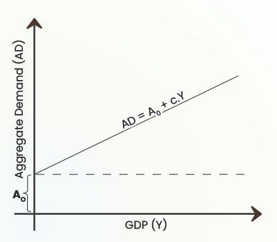

The Demand curve vs GDP curve is governed by the formula AD = A₀ + c.Y. We have seen this in the previous section in this chapter already.

Here, if the income (Y) is zero. Still, there would be certain demand in the economy.

Aggregate Supply Curve

How would the supply be governed in this economy?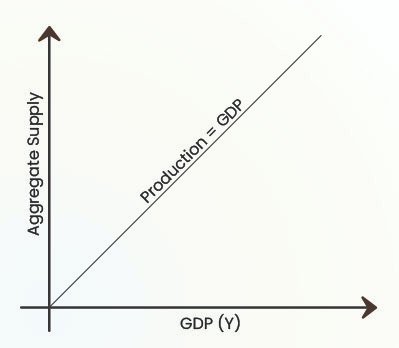 

What is supply? It is the amount of goods produced in an economy. After all, whatever is produced in the economy is available for sale. This is nothing but the supply itself.

In the previous chapter, we have learnt that the total production in an economy is referred to as the GDP.

Thus, the Supply v/s GDP graph would be a straight line angle at 45^o, signifying the aggregate supply increasing exactly as much the production increases.

Demand Supply Equilibrium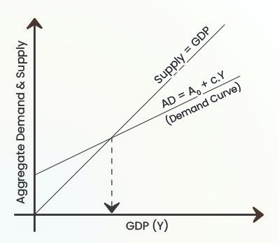

Let’s superimpose the two graphs over each other. The point where the two graphs meet signifies the equilibrium between the demand and supply.

Now this is a fun graph. It enables us to predict a few important aspects of the economy. For example:

• It tells us that for a given A₀ and c, i.e. for a given minimum demand and consumption tendency, at which level of GDP does the equilibrium occur.
• This means we can predict the GDP!

How to Increase GDP?

Now the question arises what factors should we change in order to create a favourable equilibrium that leads us to a higher GDP number?

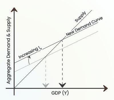
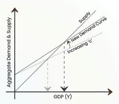
Intuition tells us that increasing demand can help us gain higher GDP because it leads to greater production.

This can happen in two ways:

1. Increasing aggregate Ex-Ante Investment.
2. Increasing consumption by increasing the marginal propensity to consume. This implies that the people consume more than they save.

 

 

 

 

 

Short-run fixed price analysis

The above analysis has been done on the basis of the Short-run fixed price analysis, also known as the effective demand principle. It assumes that the economy is capable of creating an unlimited supply. Therefore the equilibrium of output will solely be determined by the aggregate amount of demand at a fixed price.

Limitations: if the economy takes some time to respond to forces of excess supply or demand.

• The aggregate price level in the economy changes only when adjustments in all markets of the economy fail to eliminate the excess demand or supply.
• Prices are, therefore, assumed to vary only in the long run.

Income v/s Savings

There is another way to analyse the following equation. Since c is lower than 1. The aggregate demand will change slower than the level of income.

Logically, why is the growth in demand slower than the growth in income?

People always save a proportion of their income, as we have seen at the start of this chapter. Further, People save more as they earn more.

Relation between demand and income

Did you notice one thing? When the equilibrium occurs, the Supply equals demand. This demand becomes the total production in the economy, which is nothing but the GDP (as we learned in the previous chapter).

Therefore we can replace the term AD with Y, where Y is the total income/total production (GDP) of the economy.

Thus, AD = A₀ + c.Y

• Y = A₀ + c.Y
• Y – cY = A₀
• Y (1 – c) = A₀
• 

Here, remember that  “1 – c” is the marginal propensity to save (mps).

We have two implications here:

1. Incomes increase with increasing Demand (A₀)
2. Incomes decrease if people save more!!

This 2^nd implication is what causes the famous paradox of Thrift.

Paradox of Thrift:

If all the people in the economy increase the proportion of income they save (i.e. mps increases) the total value of savings in the economy will not increase – it will either decline or remain unchanged.

The Paradox of Thrift is an economic concept that highlights a potential contradiction in personal saving behaviour and its impact on the broader economy. It was first popularized by economist John Maynard Keynes.

• The paradox occurs when individuals or households increase their savings during economic downturns in an effort to secure their financial future. While this makes sense at the individual level, it can lead to negative consequences for the economy as a whole.
• When everyone in the economy attempts to save more, consumption declines, leading to reduced demand for goods and services. This reduction in demand causes businesses to cut back on production, leading to layoffs and higher unemployment. As a result, the collective increase in savings can lead to a decline in overall income and economic growth, which may counteract the intended benefits of saving.

Thus, while saving is beneficial at an individual level, if too many people save excessively at the same time, it can reduce overall economic activity, causing a contraction rather than an expansion.

FAQs related to Income Determination